Need a reliable way to pull the right value from a table without breaking formulas when columns move? This Excel XLOOKUP tutorial shows how to use XLOOKUP in Excel to replace VLOOKUP with a clearer, safer lookup formula. You’ll learn the exact syntax, how to return one value or multiple columns, and how to avoid common errors like #N/A or #SPILL!.
Introduction
If you’ve ever maintained a price list, a school project tracker, or a work spreadsheet with product IDs, you know the problem: you type an ID in one place and want Excel to automatically fill in the name, price, or department from another list. Many people solved this for years with VLOOKUP—until it started failing after “just one more” column was inserted, or when the value you needed was to the left of the ID.
XLOOKUP was created to make lookups less fragile and more readable. It can search left or right, it defaults to an exact match (so fewer silent mistakes), and it can return more than one column in a single formula in modern Excel versions. The steps below focus on everyday worksheets: a simple lookup list, a result cell, and a formula you can trust when the sheet changes later.
Basics and Overview
XLOOKUP is an Excel function that searches for a value in one range (the lookup array) and returns the matching result from another range (the return array). The key idea is that you explicitly tell Excel what to search and what to return—so you don’t rely on “the 4th column from the left” like VLOOKUP does.
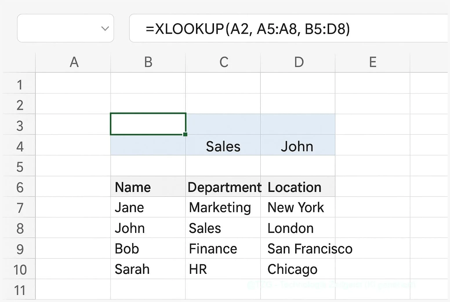
The basic syntax from Microsoft is: =XLOOKUP(lookup_value, lookup_array, return_array, [if_not_found], [match_mode], [search_mode]). The square brackets mean those arguments are optional. A practical example: look up an item number in column A, return the price from column D.
XLOOKUP is usually easier to read and harder to break, because it separates “where to search” from “what to return.”
Another big difference: XLOOKUP can return multiple adjacent columns at once in Excel versions with dynamic arrays. That result “spills” into neighboring cells automatically. If you’ve never seen that, it’s normal—the worksheet will show a highlighted spill range when it works.
| Option or Variant | Description | Suitable for |
|---|---|---|
| Basic exact match | Find a code/ID and return one value (for example, a price) with an exact match default. | Most everyday lists where the key must match exactly. |
| Return multiple columns | Return a whole row segment (for example, name and department) and let Excel spill results into adjacent cells. | Dashboards and forms where you want several fields filled at once. |
Preparation and Prerequisites
Before you convert old VLOOKUP formulas, take one minute to check your Excel environment and your data layout. XLOOKUP is available in modern Excel versions (for example Excel for Microsoft 365, Excel on the web, and recent perpetual versions such as Excel 2021). If you share files with people on older Excel releases, they may see #NAME? instead of results because their Excel doesn’t know XLOOKUP.
Use this quick checklist so your first XLOOKUP works right away:
- Confirm your key column is clean: IDs should be consistent (no mixed formats like “0012” vs “12”). Remove leading/trailing spaces if needed.
- Make sure lookup and return ranges line up: If your lookup array has 100 rows, your return array must cover the same 100 rows.
- Decide what should happen when nothing is found: Plan a friendly message like “Not found” via if_not_found instead of showing #N/A.
- If you want multiple columns back: Reserve empty cells to the right (or below) for the spill output, otherwise you may trigger #SPILL!.
If you work with structured data often, consider first turning your list into an Excel Table (Ctrl+T on Windows, Cmd+T on macOS). Tables make ranges expand automatically when you add new rows.
Step-by-Step Instruction
The example below assumes you have a small “database” list with a unique key (like Product ID) and you want to fill details into another area. The steps are identical whether you’re replacing VLOOKUP in an old file or building a new sheet.
- Identify the lookup value cell. Click the cell that contains the key you will search for (for example, E2 with a Product ID). If the ID is typed by a person, consider Data Validation later to reduce typos.
- Select where the result should appear. Click the output cell (for example, F2 for the product name). This is where you’ll enter the formula.
- Start the XLOOKUP formula. Type =XLOOKUP( and then click the lookup value cell (E2). Excel will insert it into the formula.
- Set the lookup array. Select the column (or range) that contains the IDs in your list, for example A2:A200. This is the list XLOOKUP searches in.
- Set the return array. Select the column (or range) you want to return from, for example C2:C200 for a name. Your basic formula now looks like: =XLOOKUP(E2, A2:A200, C2:C200).
- Add a friendly not-found message (recommended). After the return array, add a fourth argument such as “Not found”. Example: =XLOOKUP(E2, A2:A200, C2:C200, “Not found”).
- Copy the formula down (if needed). Use the fill handle (small square at the cell corner) to copy it to other rows, or turn your output area into a Table column so formulas auto-fill.
- Optional: return multiple columns in one go. If you want Name and Price together, set the return array to a multi-column range like C2:D200. Enter it in the leftmost output cell (for example F2). In modern Excel, the results will spill into adjacent cells automatically.
If everything is correct, the output cell immediately shows the matching value. If you returned multiple columns, you should see a filled block of cells and a subtle spill outline around it. When you change the ID, the results update instantly.
Tips, Troubleshooting, and Variants
If XLOOKUP doesn’t behave as expected, it’s usually a data mismatch, a blocked spill area, or a version/compatibility issue. These fixes solve most real-world cases without getting overly technical.
Common issues and quick fixes
- You get #N/A (or your “Not found” message appears too often): Check if the key values really match. A frequent problem is hidden spaces or different data types (number vs text). Cleaning the key column often resolves this.
- You see #SPILL! when returning multiple columns: Something blocks the cells where Excel wants to place the spilled results. Clear those cells, unmerge merged cells, or move the formula to an area with enough empty space. Microsoft documents #SPILL! causes and fixes in detail.
- Someone else sees #NAME? in the shared file: Their Excel version likely doesn’t support XLOOKUP. For shared templates across mixed versions, keep a fallback approach (often INDEX/MATCH) or agree on a minimum Excel version.
Practical variants you’ll use often
- Search from the bottom: If your list contains duplicates and you want the last match (for example, the most recent entry), use the optional search_mode of -1 to search last-to-first.
- Wildcard search for messy inputs: With match_mode set to 2, XLOOKUP supports wildcards like * and ? (useful when you only know part of a name). Use carefully, because it can match more than you expect.
- Make your sheet more robust: Combine XLOOKUP with an input dropdown to avoid typos. If you want, follow TechZeitGeist’s guide on Excel drop-down lists with Data Validation.
- Pair lookups with quick analysis: After you pull the right fields with XLOOKUP, a PivotTable is a simple next step for summaries. TechZeitGeist also explains how to build a PivotTable fast.
Tip for readability: if your XLOOKUP starts to look long, add line breaks in the formula bar (Alt+Enter on Windows) and keep your ranges consistent. Clear formulas are easier to maintain than “clever” ones.
Conclusion
XLOOKUP is a practical upgrade for everyday spreadsheets: you choose the search range and the return range explicitly, so your lookup doesn’t depend on a fragile column number. That makes it a strong replacement for VLOOKUP when lists change over time. With an optional not-found message, your sheet also becomes friendlier for other people. If you work in a modern Excel version, returning multiple columns can reduce repeated formulas and keep dashboards tidy. Once you’ve set up one clean XLOOKUP, copying and reusing it becomes straightforward.
Try replacing one VLOOKUP you rely on most and note what becomes simpler—then share your biggest “gotcha” (or your cleanest setup) with others.


Leave a Reply