An Excel drop-down list keeps spreadsheets clean: instead of typing, you pick a value from a menu so names, statuses, or categories stay consistent. This tutorial shows how to build an Excel Data Validation list that is easy to maintain, can pull options from another sheet, and guides users with helpful messages. You will end with a working drop-down, plus a few safe variants for real-world files.
Introduction
Many Excel files fail for a simple reason: people type the same thing in different ways. “In progress” becomes “in-progress”, “In Progress”, or “IP”. A city name is misspelled once, and filters and pivot tables suddenly look wrong. In shared workbooks, this happens fast—especially when the sheet acts like a small form for orders, tickets, inventories, or class lists.
A drop-down list solves that everyday problem by limiting what can be entered in certain cells. In Excel, this is done with Data Validation, a built-in rule system that can offer a list of allowed values and show guidance or an error message if someone tries to type something else.
The steps below work in current Excel versions on Windows and macOS. The menus may look slightly different, but the names are very similar.
Basics and Overview: the Excel drop-down list (Data Validation)
An Excel drop-down list is not a separate “widget”. It is a rule applied to one or more cells: Excel checks the input and, if the rule is a list, it shows a small arrow in the cell. When you click it, you can pick one of the allowed items.
The key term is Data Validation. Think of it as a bouncer for your cells: it decides what is allowed in, and what gets rejected. A Data Validation List can be based on (1) items typed directly into the rule, (2) a cell range, or (3) a named range (a range with a memorable name you can reuse across the workbook).
The most maintainable drop-down lists are built from a dedicated list range (often on another sheet), not from values typed into the validation dialog.
When the source list lives on its own sheet, you can update options without touching the validated cells. This is especially helpful for team spreadsheets. If you want a deeper Excel workflow mindset, TechZeitGeist also covers common spreadsheet hygiene patterns in its Excel guides, for example creating Excel drop-down lists with Data Validation.
| Option or Variant | Description | Suitable for |
|---|---|---|
| List from a cell range | Source is a fixed range like Lists!A2:A20. | Small, stable lists you rarely change. |
| List from a named range / table | Source is a name like =StatusList (often backed by a table that grows). | Lists that will change over time and should be easy to maintain. |
Preparation and Prerequisites
Before you build the drop-down, set up your list values in a clean way. This prevents most issues later—especially in shared workbooks.
Preparation checklist:
- Decide where the list lives: ideally in a separate worksheet (for example a sheet named Lists).
- Use one item per cell in a single column, with no empty rows inside the list.
- Remove leading/trailing spaces in the list items (spaces can create “different” values that look identical).
- Check your permissions: if the workbook or sheet is protected, you may need to unprotect it to change Data Validation rules.
- Think about maintenance: if the list may grow, consider converting it into an Excel table (Select the list and press Ctrl+T on Windows or Cmd+T on macOS). Tables automatically expand when you add new items.
If your list should come from another sheet: that is fine, but the cleanest approach is to create a named range (or name the table column) and use that name as the source. Microsoft’s guidance commonly recommends named ranges for easier updates across a workbook.
Step-by-Step Instruction
The steps below create a classic drop-down list using Data Validation and a named range, which works well across sheets and is easier to maintain than a hard-coded range.
- Create the source list. On a worksheet such as Lists, type your options in a single column (example: A2:A10 contains statuses like “New”, “In progress”, “Done”).
- Name the list range. Select the cells that contain your items. Then open Formulas > Define Name (or Name Manager). Give it a clear name without spaces, for example StatusList, and confirm. (This is your reusable source.)
- Select the target cells. Go to the sheet where users will enter data and highlight the cells that should get the drop-down (for example, column D in a table of tasks).
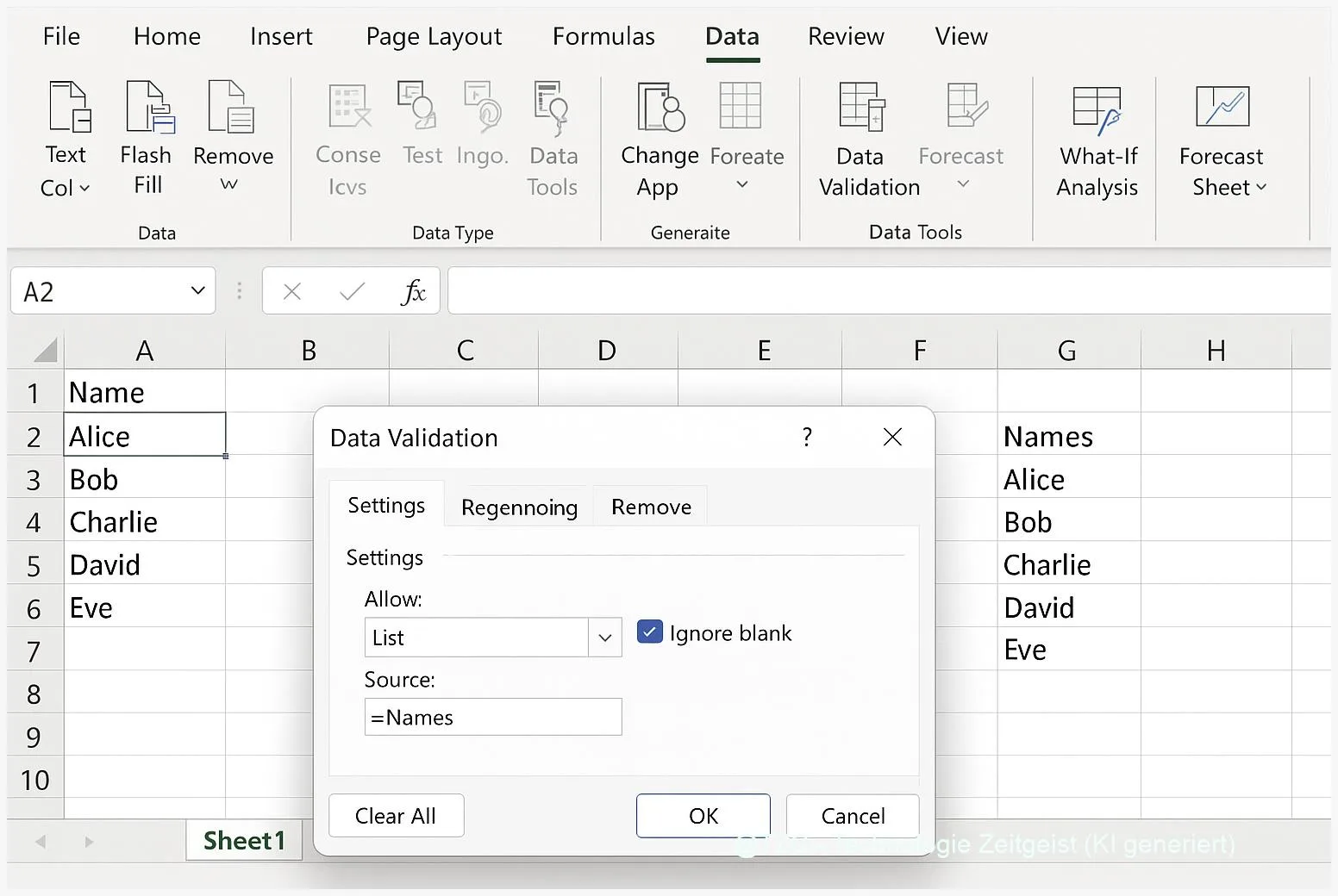
- Open Data Validation. Go to Data > Data Validation. If you see a small dialog launcher icon, click it to open the full settings.
- Set the rule to a list. In the settings, choose Allow: List. In Source, enter =StatusList (with the equals sign). Confirm.
- Optional: add a helpful hint. In the Input Message tab, enable the message and write something short like “Pick a status from the list”. This appears when the cell is selected.
- Optional: configure a clear error message. In Error Alert, keep the style strict (often Stop) and use a friendly text like “Please choose a value from the drop-down list.”
- Test it. Click one of the validated cells. You should see a small drop-down arrow. Choose an item and confirm it appears exactly as written in the list.
If everything is set up correctly, the drop-down arrow appears when the cell is active, and typing an invalid value triggers your error message (depending on the chosen alert style).
Tips, Troubleshooting, and Variants
Even a simple drop-down can behave “oddly” when a workbook is large, shared, or edited over time. These fixes cover the most common stumbling blocks.
The drop-down arrow does not show:
- Re-select a validated cell (the arrow usually appears only when the cell is active).
- Open Data Validation again and confirm that In-cell dropdown is enabled.
- Check if the sheet is protected in a way that blocks selecting unlocked cells or editing validation rules.
The list does not include new items:
- If you used a fixed range, extend the range (or switch to a table-backed named range).
- If you used a named range, open Name Manager and verify that the “Refers to” range includes the new rows.
Variant: drop-down list from another sheet (without naming). You can point Data Validation directly at a range on a different worksheet, but it is easier to break during edits. A named range is usually the safer long-term option.
Variant: simple dependent (cascading) drop-downs. In some workflows, the second drop-down depends on the first (for example: Category → Subcategory). One common technique uses named ranges plus the INDIRECT function (it turns text into a reference). This can work well, but it also adds complexity and may slow down very large workbooks because INDIRECT is a volatile function. Consider it only if you truly need it and document your naming rules clearly.
Data quality tip: After adding Data Validation to an existing sheet, old entries may still be inconsistent. Microsoft’s Data Validation guidance includes tools such as circling invalid data, which helps you find and clean up cells that don’t match your new rules.
Conclusion
An Excel drop-down list is one of the simplest ways to prevent messy data without turning a spreadsheet into a rigid system. With a clean source list and an Excel Data Validation list, you guide users toward consistent values, reduce typos, and make filtering and reporting far more reliable. The most practical setup is a list stored on its own sheet and connected via a named range, so updates stay easy even months later. Once you get used to it, you will start adding drop-downs to any sheet that is filled out repeatedly.
Try adding one drop-down to a real sheet you use weekly—and share what worked (or what broke) so others can learn from your setup.


Leave a Reply